Module 48 for loops
Learning goals
- What
forloops are, and how to use them yourself
- How to use
forloops to carry out repetitive analyses
- How to use
forloops to summarize subgroups in your data
- How to use
forloops to create and work with many data files at once
- How to use
forloops for plots that are tricky but cool
- How to use nested
forloops
Basics
A for loop is a super powerful coding tool. In a for loop, R loops through a chunk of code for a set number of repititions.
A super basic example:
Here’s an example of a pretty useless for loop:
for(i in 1:5){
  print("I'm just repeating myself.")
}
[1] "I'm just repeating myself."
[1] "I'm just repeating myself."
[1] "I'm just repeating myself."
[1] "I'm just repeating myself."
[1] "I'm just repeating myself."
This code is saying:
- For each iteration of this loop, step to the next value in x (first example) or 1:5 (second example).
- Store that value in an object i,
- and run the code inside the curly brackets.
- Repeat until the end of x.
Look at the basic structure:
- In thefor( ) parenthetical, you tell R what values to step through (x), and how to refer to the value in each iteration (i).
- Within the curly brackets, you place the chunk of code you want to repeat.
Another basic example, demonstrating that you can update a variable repeatedly in a loop.
Silly example 1:
professors <- c("Keri","Deb","Ken")
for(x in professors){
  print(paste0(x," is pretty cool!"))
}
[1] "Keri is pretty cool!"
[1] "Deb is pretty cool!"
[1] "Ken is pretty cool!"
Silly example 2:
professors <- c("Keri","Deb","Ken")
claims <- c()
for(x in professors){
  claim_x <- paste0(x," is pretty cool!")
  claims <- c(claims, claim_x)
}
claims
[1] "Keri is pretty cool!" "Deb is pretty cool!"  "Ken is pretty cool!"
“Nested” for loops:
x <- 1:5
y <- 6:10
for(i in x){
  for(j in y){
  print(paste0(i,"-",j))
  }
}
[1] "1-6"
[1] "1-7"
[1] "1-8"
[1] "1-9"
[1] "1-10"
[1] "2-6"
[1] "2-7"
[1] "2-8"
[1] "2-9"
[1] "2-10"
[1] "3-6"
[1] "3-7"
[1] "3-8"
[1] "3-9"
[1] "3-10"
[1] "4-6"
[1] "4-7"
[1] "4-8"
[1] "4-9"
[1] "4-10"
[1] "5-6"
[1] "5-7"
[1] "5-8"
[1] "5-9"
[1] "5-10"
for loop workflow
Loops can be simple or complex, but the procedure for building any for loop is the same. The general idea is to write the body of your loop first, test it to make sure it works, then wrap it in a for loop. Use the code below as a template for building for loops.
# Step 1. Give 'i' an arbitrary value for the time being
i=1

# Step 2. If needed, stage empty plots or objects here.


# Step 5. Open up your `for` loop here.


# Step 3. Write the body of your loop


# Step 4. Test the code you wrote for Step 2 (i.e., run the code for Steps 1 and 2).


# Step 6. Close your `for` loop with an end curly bracket.
for loop exercises
Use case 1: Repetitive printing
1a. Practice using the for loop template to make your own version of silly example 1.
1b. Practice the for loop template to make your own version of silly example 2.
1c. Pretend you are doing a big repetitive analysis with 1,000 iterations. Pretend each iteration takes a long time to process, so it would be nice to print a status update each time an iteration is complete. Write a for loop that prints a status update with each iteration (e.g., “Iteration 3 out of 1,000 is complete …”).
Use case 2: Self-building calculations
2a. Create a vector with these values: 45, 245, 202, 858, 192, 202, 121. Build a for loop that prints the cumulative sums for this vector. (If your vector is 1,1,3, then the cumulative sums are 1,2,5.)
2b. Modify this for loop so that the cumulative sums are saved to a second vector object, instead of printed to the console.
(Note: there is a built-in function, cumsum(), that you can also use for this application)
Use case 3: Summarizing subgroups in your data
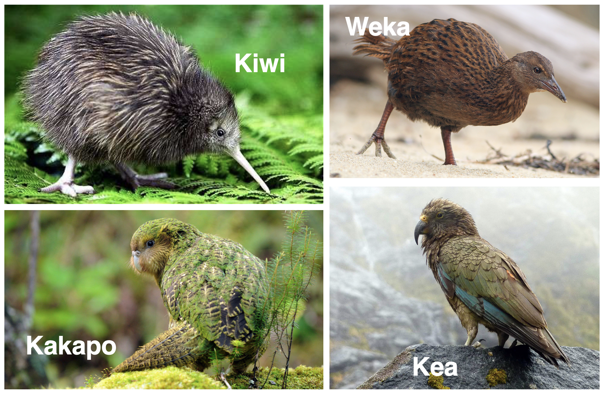
Scenario: You participate in a survey of flightless birds in the forests of New Zealand. You conduct thirty days of fieldwork on four species of bird: the kiwi, the weka, the kakapo (the world’s heaviest parrot), and the kea (the world’s only alpine parrot).
Download the data, place it in your working directory, and read it into your R session.
Your data (nz_birds.csv) look like this:
df <- read.csv("./data/nz_birds.csv")
nrow(df)
[1] 406
head(df)
  day species group
1   1    Kiwi     3
2   1     Kea     4
3   1  Kakapo     4
4   1    Weka     2
5   1    Kiwi     1
6   1     Kea     3
tail(df)
    day species group
401  30    Weka     3
402  30    Kiwi     3
403  30    Kiwi     3
404  30  Kakapo     3
405  30  Kakapo     1
406  30     Kea     2
Each row contains the data for a single bird group detection.
Your supervisor has asked you to write a report of your findings. In that report she wants to see a table with the number of each species seen on each day of the fieldwork. That table will look something like this:
  day kiwi weka kakapo kea
1   1    5    6      3   3
2   2    1    3      1   2
3   3    2    4      5   3
4   4    2    3      2   0
5   5    6    6      3   2
6   6    6    2      3   6
Use a for loop to create this table.
Note that this is a very common use case for for loops. Other examples of this use case include these scenarios:
You want to summarize sample counts for each day of fieldwork.
You want to summarize details for each user in your database.
You want to summarize weather information for each month of the year.
Use case 4: Repetitive file creation
Scenario, continued: Your supervisor also wants to be able to share a public version of the New Zealand survey data with some of her collaborators. Rather than share the raw data, she would like to have a separate data file for each species of bird. Use a for loop to create a data file (.csv format) for each bird species.
Hint: First, set your working directory. Then, within your working directory, create a folder where you can deposit the files you create.
Use case 5: Reading in multiple files
In the previous use case, you divided your original dataset into several files. Now see if you can write a for loop that reverses the process. In other words, build a for loop that combines several data files into a single dataframe.
Hint: Recall that you can use the function rbind() to combine two or more dataframes.
Use case 6: Layering cyclical data on a plot
First, read in some cool data (keeling-curve.csv).
kc <- read.csv("./data/keeling-curve.csv") ; head(kc)
  year month day_of_month day_of_year year_dec frac_of_year    CO2
1 1974     5           26    145.4890 1974.399       0.3986 332.95
2 1974     6            2    152.4970 1974.418       0.4178 332.35
3 1974     6            9    159.5050 1974.437       0.4370 332.20
4 1974     6           16    166.5130 1974.456       0.4562 332.37
5 1974     6           23    173.4845 1974.475       0.4753 331.73
6 1974     6           30    180.4925 1974.495       0.4945 331.68
This is the famous Keeling Curve dataset: long-term monitoring of atmospheric CO2 measured at a volcanic observatory in Hawaii.
Try plotting the Keeling Curve:
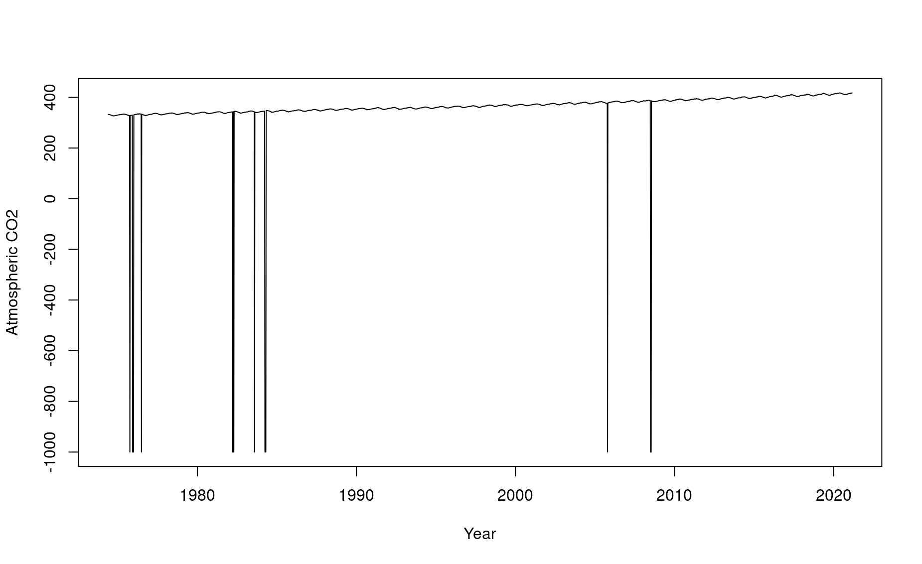
There are some erroneous data points! We clearly can’t have negative CO2 values. Let’s remove those and try again:
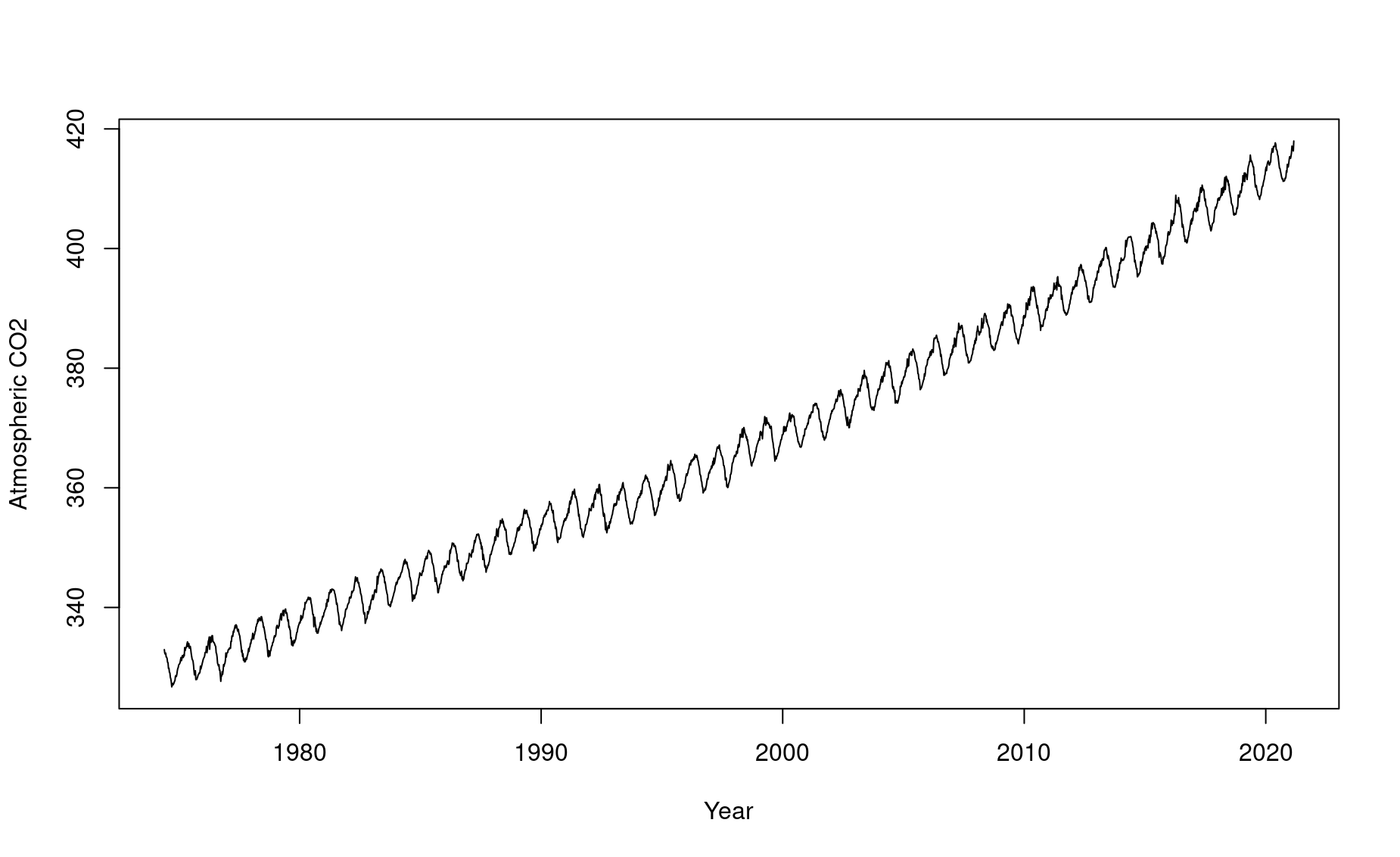
What’s the deal with those squiggles? They seem to happen every year, cyclically. Let’s investigate!
Let’s look at the data a different way: by layering years on top of one another.
To begin, let’s plot data for only a single year:
# Stage an empty plot for what you are trying to represent
plot(1, # plot a single point
     type="n",
     xlim=c(0,365),xlab="Day of year",
     ylim=c(-5,5),ylab="CO2 anomaly")
abline(h=0,col="grey") # add nifty horizontal line

# Reduce the dataset to a single year (any year)
kcy <- kc[kc$year=="1990",] ; head(kcy)
    year month day_of_month day_of_year year_dec frac_of_year    CO2
816 1990     1            7      6.4970 1990.018       0.0178 353.58
817 1990     1           14     13.5050 1990.037       0.0370 353.99
818 1990     1           21     20.5130 1990.056       0.0562 353.92
819 1990     1           28     27.4845 1990.075       0.0753 354.39
820 1990     2            4     34.4925 1990.094       0.0945 355.04
821 1990     2           11     41.5005 1990.114       0.1137 355.09

# Let's convert each CO2 reading to an 'anomaly' compared to the year's average.
CO2.mean <- mean(kcy$CO2,na.rm=TRUE) ; CO2.mean  # Take note of how useful that 'na.rm=TRUE' input can be!
[1] 354.4538

y <- kcy$CO2 - CO2.mean ; y # Translate each data point to an anomaly
 [1] -0.87384615 -0.46384615 -0.53384615 -0.06384615  0.58615385  0.63615385
 [7]  0.96615385  0.72615385  1.13615385  1.33615385  1.08615385  1.67615385
[13]  1.81615385  1.71615385  1.77615385  2.41615385  2.50615385  3.24615385
[19]  2.79615385  2.87615385  2.92615385  2.52615385  1.79615385  1.72615385
[25]  1.33615385  1.76615385  0.53615385 -0.16384615 -0.08384615 -0.46384615
[31] -1.28384615 -0.99384615 -1.37384615 -2.65384615 -3.29384615 -3.59384615
[37] -2.70384615 -2.99384615 -3.05384615 -2.91384615 -2.88384615 -2.72384615
[43] -2.05384615 -1.74384615 -1.30384615 -1.00384615 -0.76384615 -0.55384615
[49]  0.01615385 -0.11384615  0.37615385  0.34615385          NA

# Add points to your plot
points(y~kcy$day_of_year,pch=16,col=adjustcolor("darkblue",alpha.f=.3))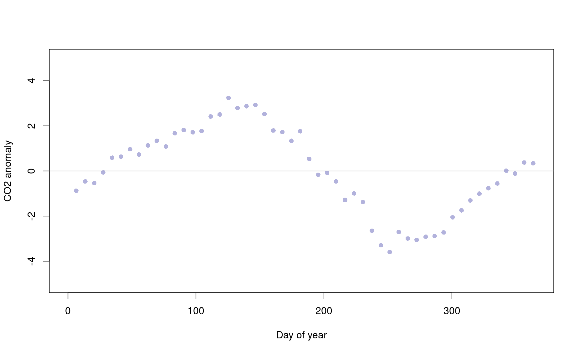
But this only shows one year of data! How can we include the seasonal squiggle from other years?
Figure out how to use a for loop to layer each year of data onto this plot. Your final plot will look like this:
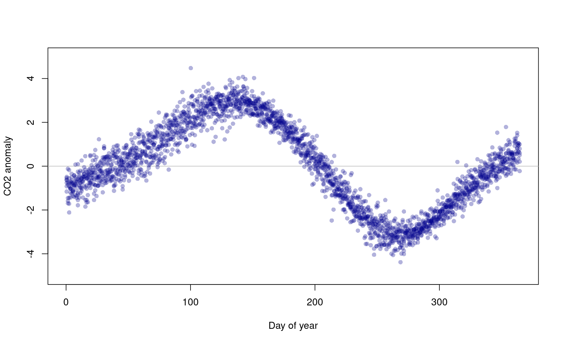
So how do you interpret this graph? Why do you think those squiggles happen every year?
Other use cases for plots
Efficient multi-panel plots
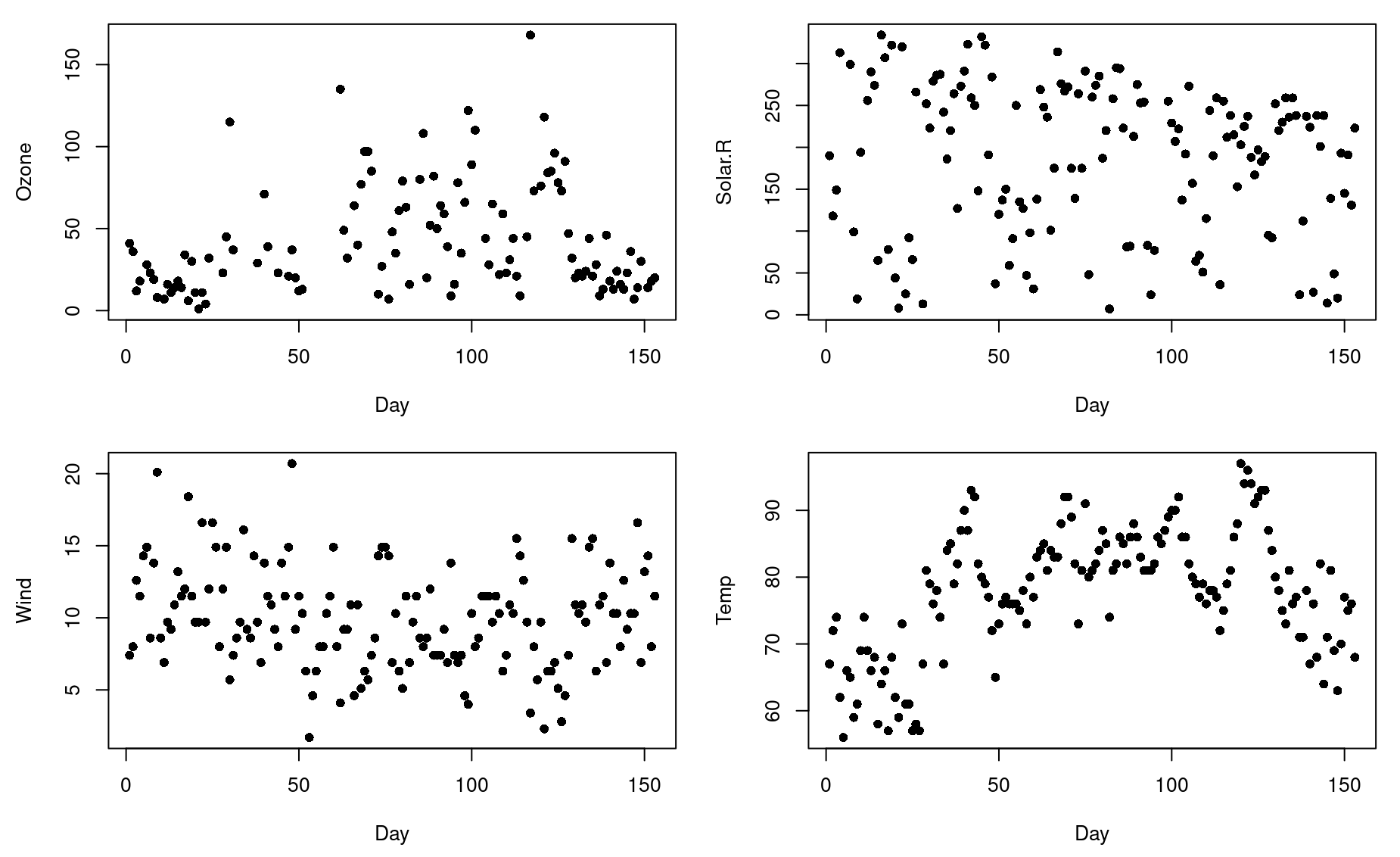
A for loop can be a very efficient way of making multi-panel plots.
Let’s use a for loop to get a quick overview of the variables included in the airquality dataset built into R.
data(airquality)
head(airquality)
  Ozone Solar.R Wind Temp Month Day
1    41     190  7.4   67     5   1
2    36     118  8.0   72     5   2
3    12     149 12.6   74     5   3
4    18     313 11.5   62     5   4
5    NA      NA 14.3   56     5   5
6    28      NA 14.9   66     5   6
Looks like the first four columns would be interesting to plot.
par(mfrow=c(2,2)) # Setup a multi-panel plot # format = c(number of rows, number of columns)
par(mar=c(4.5,4.5,1,1)) # Set plot margins

# Loop through the first four columns ...
for(i in 1:4){
  y <- airquality[,i] # Select data in column i
  var.name <- names(airquality)[i] # Get name of that column
  plot(y,xlab="Day",ylab=var.name,pch=16) # Plot data
}
Using for loops to plot subgroups of data
for loops are also useful for plotting data in tricky ways. Let’s use a different built-in dataset, that shows the performance of various car make/models.
data(mtcars)
head(mtcars)
mpg cyl disp hp drat wt qsec vs am gear carb
Mazda RX4 21.0 6 160 110 3.90 2.620 16.46 0 1 4 4
Mazda RX4 Wag 21.0 6 160 110 3.90 2.875 17.02 0 1 4 4
Datsun 710 22.8 4 108 93 3.85 2.320 18.61 1 1 4 1
Hornet 4 Drive 21.4 6 258 110 3.08 3.215 19.44 1 0 3 1
Hornet Sportabout 18.7 8 360 175 3.15 3.440 17.02 0 0 3 2
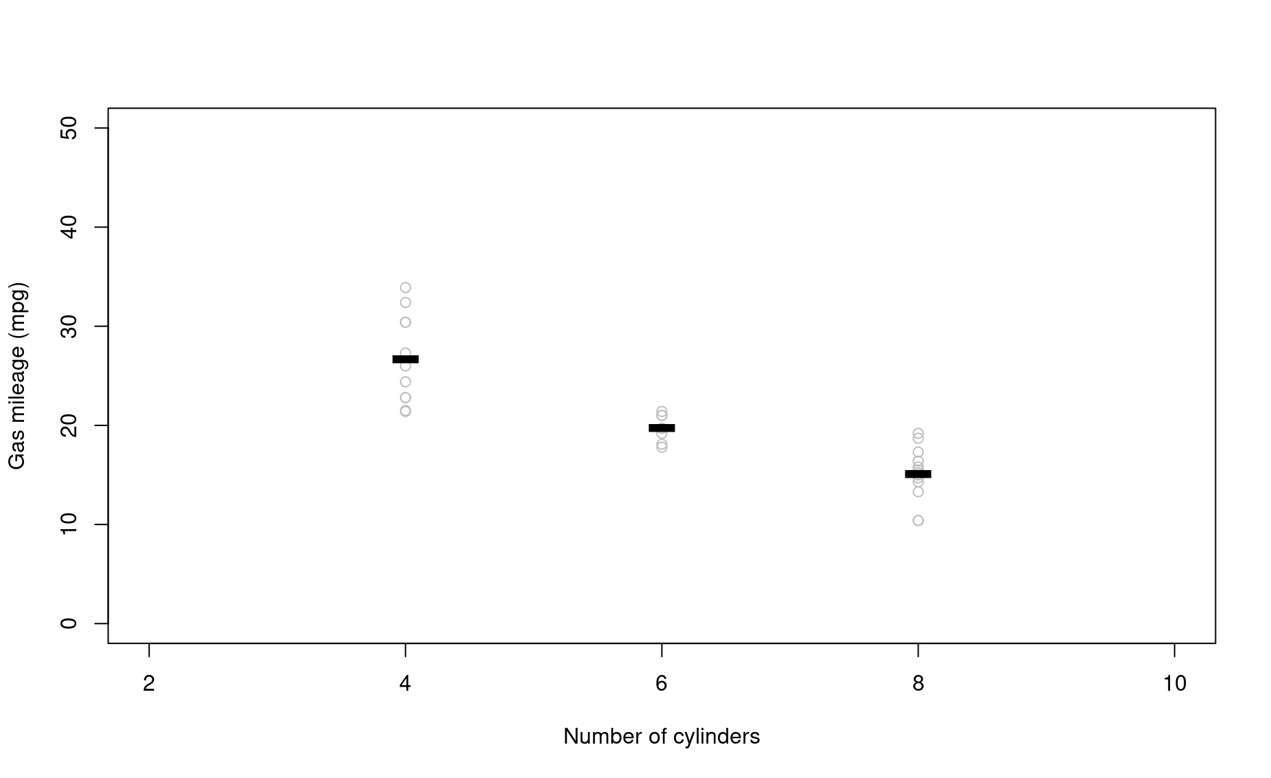
Valiant 18.1 6 225 105 2.76 3.460 20.22 1 0 3 1Let’s say we want to see how gas mileage is affected by the number of cylinders a car has. It would be nice to create a plot that shows the raw data as well as the mean mileage for each cylinder number.
# Let's see how many different cylinder types there are in the data
ucyl <- unique(mtcars$cyl) ; ucyl
[1] 6 4 8

# Let's make an empty plot
plot(1,type="n", # tell R not to draw anything
     xlim=c(2,10),ylim=c(0,50),
     xlab="Number of cylinders",
     ylab="Gas mileage (mpg)")

# Write your for loop here to add the actual data

i=ucyl[1] # It's always good to use a known value of i as you build up your for loop

for(i in ucyl){ # Usually helpful to write this line LAST.
                # i.e., write body of loop first, test it, then wrap it in a loop.

  # Subset the dataframe according to number of cylinders
  cari <- mtcars[mtcars$cyl==i,]

  # Plot the raw data
  points(x=cari$cyl,y=cari$mpg,col="grey")

  # Superimpose the mean on top
  points(x=i,y=mean(cari$mpg),col="black",pch="-",cex=5,)
}
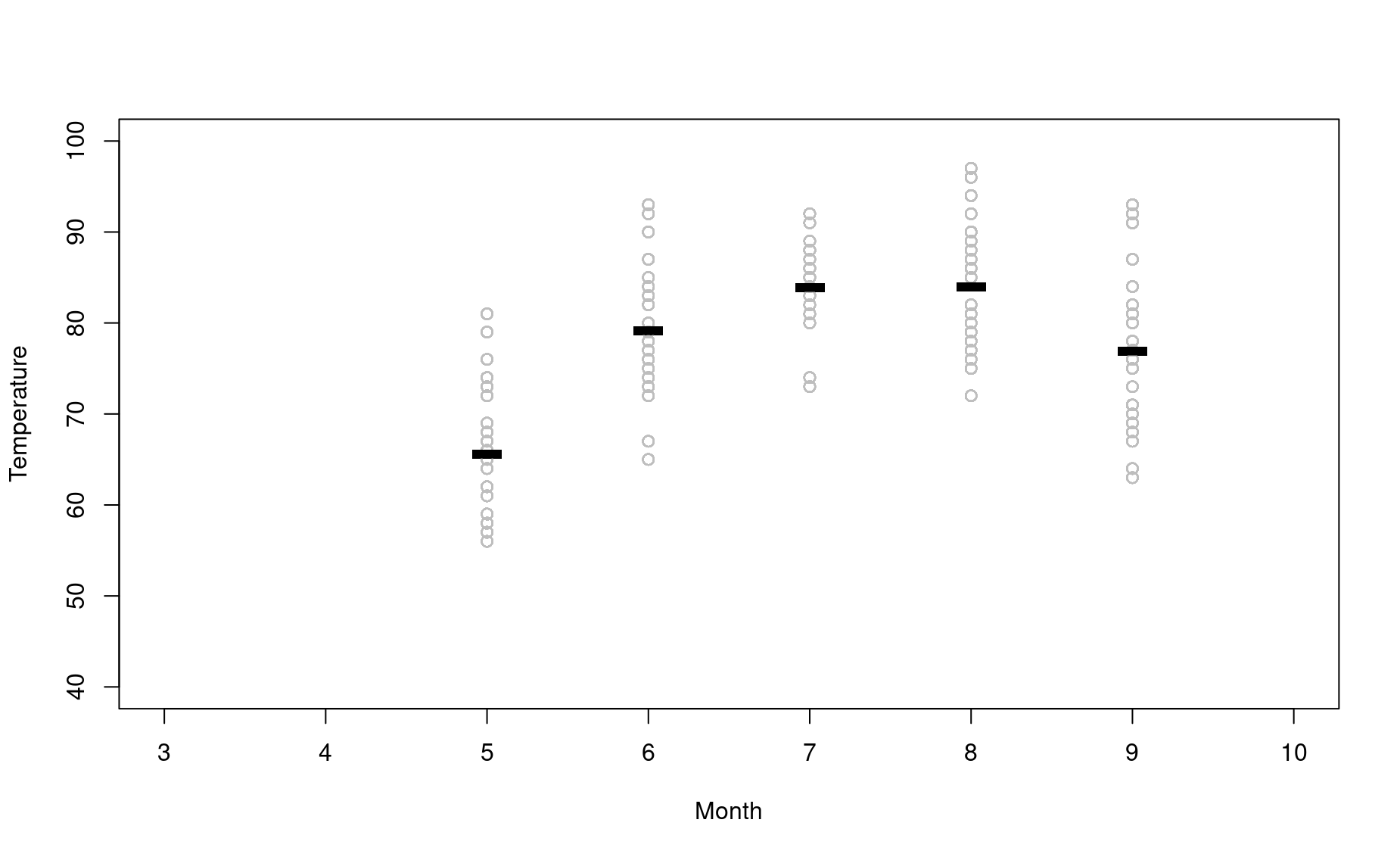
Now try to do something similar on your own with the airquality dataset. Use for loops to create a plot with Month on the x axis and Temperature on the y axis. On this plot, depict all the temperatures recorded in each month in the color grey, then superimpose the mean temperature for each month.
We will provide the empty plot, you provide the for loop:
plot(1,type="n",
     xlim=c(3,10),ylim=c(40,100),
     xlab="Month",
     ylab="Temperature")

# Write your for loop here to add the actual data
for(i in airquality$Month){
  airi <- airquality[airquality$Month==i,]
  points(x=airi$Month,y=airi$Temp,pch=1,col="grey")
  points(x=i,y=mean(airi$Temp),pch="-",cex=5,col="black")
}
Review assignments
Review assignment 1
Sometimes you need to summarize your data in such a specific way that you will need to use nested for loops, i.e., one for loop contained within another.
For example, your supervisor for the New Zealand Flightless Birds Survey has now taken an interest in associations among the four bird species you have been monitoring. For example, are kiwis more abundant on the days when you detect a lot of kakapos?
To answer this question, your supervisor wants to see a table with each species combination (Kiwi - Kakapo, Kiwi - Weka, … Kakapo - Kea, etc.) and the number of dates in which both species were seen more than 5 times.
You can produce this table using a nested for loop. Here is how it’s done:
uspp <- unique(df$species) # get set of unique species

A <- B <- c() # empty vector for names of each species in the pair
X <- c() # empty vector for number of dates in which both species were common

i=1 ; j=2

# For loop 1
for(i in 1:length(uspp)){
  spi <- uspp[i] # species i
  dfi <- df[df$species == spi,] # subset df to only this species
  counti <- table(dfi$day) # get number of sightings on each day
  dayi <- names(counti)[which(counti >= 5)] ; # get the dates on which this species was seen 5+ times

  # For loop 2
  for(j in 1:length(uspp)){
    spj <- uspp[j] # species j
    dfj <- df[df$species == spj,] # subset df to only this species
    countj <- table(dfj$day) # get number of sightings on each day
    dayj <- names(countj)[which(countj >= 5)] ; # get the dates on which this species was seen 5+ times

    dates_ij <- which(dayi  %in% dayj) # get the dates on which both species were seen 5+ times
    Xij <- length(dates_ij) # count the number of these dates

    # Add results to staged objects
    X <- c(X,Xij)
    A <- c(A,spi)
    B <- c(B,spj)
  }

}

# Combine results into a dataframe
results <- data.frame(A, B, X)

# Check it out!
results
        A      B  X
1    Kiwi   Kiwi  7
2    Kiwi    Kea  3
3    Kiwi Kakapo  1
4    Kiwi   Weka  3
5     Kea   Kiwi  3
6     Kea    Kea 10
7     Kea Kakapo  3
8     Kea   Weka  2
9  Kakapo   Kiwi  1
10 Kakapo    Kea  3
11 Kakapo Kakapo  7
12 Kakapo   Weka  1
13   Weka   Kiwi  3
14   Weka    Kea  2
15   Weka Kakapo  1
16   Weka   Weka  8
Note that the code for adding the results to the staged objects X, A, and B is contained within the second for loop. This is necessary for producing our results; if we put that code in the first for loop after the code for the nested loop, our results would not be complete.
Note that each for loop must use a different variable to represent each iteration. In this example, the first loop uses i and the second uses j. If we used i for both loops, R would get very confused indeed.
Also note that we used i and j in the variables specific to each loop (e.g., dayi and dayj), as a simple way to help us keep track of what each variable is representing.
Review assignment 2
Your supervisor is happy with your pairwise species association dataframe, and wants to use it in an analysis for a publication. However, the R package she wants to use requires that the data be in the format of a square matrix with four rows – one for each species – and four columns. Like this:
results_matrix <- matrix(data=NA, nrow=4, ncol=4, dimnames=list(uspp,uspp))
results_matrix
       Kiwi Kea Kakapo Weka
Kiwi     NA  NA     NA   NA
Kea      NA  NA     NA   NA
Kakapo   NA  NA     NA   NA
Weka     NA  NA     NA   NA
You have not yet worked with matrices in this curriculum (you will in a few modules), but for now think of them as simple dataframes with a single type of data (e.g., all numeric values, like this one). You can subset matrices just as you would a dataframe: matrix[row,column].
The values in this matrix should represent the number of dates in which each species pair was seen 5 times or more. For example, result[1,2] would be 3, since the Kiwi and Kea were seen 5+ times on only 3 dates.
She asks you to use the dataframe you just created to create this matrix. Use a nested for loop to do it.
# Stage empty results objects
results_matrix <- matrix(data=NA, nrow=4, ncol=4, dimnames=list(uspp,uspp))

# Get unique species
uspp <- unique(c(results$A,results$B))

# Loop 1: each species (row)
for(i in 1:length(uspp)){
  spi <- uspp[i]
  resultsi <- results[results$A==spi,] # subset data to rows where column A equals species i

  # Loop 2: each species (column)
  for(j in 1:length(uspp)){
    spj <- uspp[j]
    resultsj <- resultsi[resultsi$B==spj,] # subset data from i loop where column B equals species j

    Xij <- resultsj$X      # Find result

    results_matrix[i,j] <- Xij     # Add result to staged object
  }
}

results_matrix
       Kiwi Kea Kakapo Weka
Kiwi      7   3      1    3
Kea       3  10      3    2
Kakapo    1   3      7    1
Weka      3   2      1    8
Boom!
Review assignment 3
First, read in and format some other cool data (renewable-energy.csv). The code for doing so is provided for you here:
This dataset, freely available from World Bank, shows the renewable electricity output for various countries, presented as a percentage of the nation’s total electricity output. They provide this data as a time series.
Summarize columns with a for loop
Task 3A: Use a for loop to find the change in renewable energy output for each nation in the dataset between 1990 and 2015. Print the difference for each nation in the console.
# Write your code here
i=2
for(i in 2:ncol(df)){
  dfi <- df[,i] ; dfi
  diffi <- dfi[length(dfi)] - dfi[1] ; diffi
  print(paste0(names(df)[i]," : ",round(diffi),"% change."))
}
[1] "World : 3% change."
[1] "Australia : 4% change."
[1] "Canada : 1% change."
[1] "China : 4% change."
[1] "Denmark : 62% change."
[1] "India : -9% change."
[1] "Japan : 5% change."
[1] "New_Zealand : 0% change."
[1] "Sweden : 12% change."
[1] "Switzerland : 7% change."
[1] "United_Kingdom : 23% change."
[1] "United_States : 2% change."
Task 3B: Re-do this loop, but instead of printing the differences to the console, save them in a vector.
# Write your code here
diffs <- c()
i=2
for(i in 2:ncol(df)){
  dfi <- df[,i] ; dfi
  diffi <- dfi[length(dfi)] - dfi[1] ; diffi
  diffs <- c(diffs,diffi)
}
diffs
 [1]  3.49241703  3.98181045  0.63273122  3.51887728 62.33064943 -9.14624362
 [7]  4.73004321  0.07524008 12.26263811  7.21543884 23.01128298  1.69994636
Multi-pane plots with for loops
Practice with a single plot
Task 3C: First, get your bearings by figuring out how to use the df dataset to plot the time series for the United States, for the years 1990 - 2015. Label the x axis “Year” and the y axis “% Renewable”. Include the full name of the county as the main title for the plot.
# Write code here
dfi <- df[,c(1,13)]
plot(x=dfi[,1],
     y=dfi[,2],
     type="l",lwd=2,
     xlim=c(1990,2015),ylim=c(0,100),
     xlab="Year",ylab="% renewable",
     main=names(dfi)[2])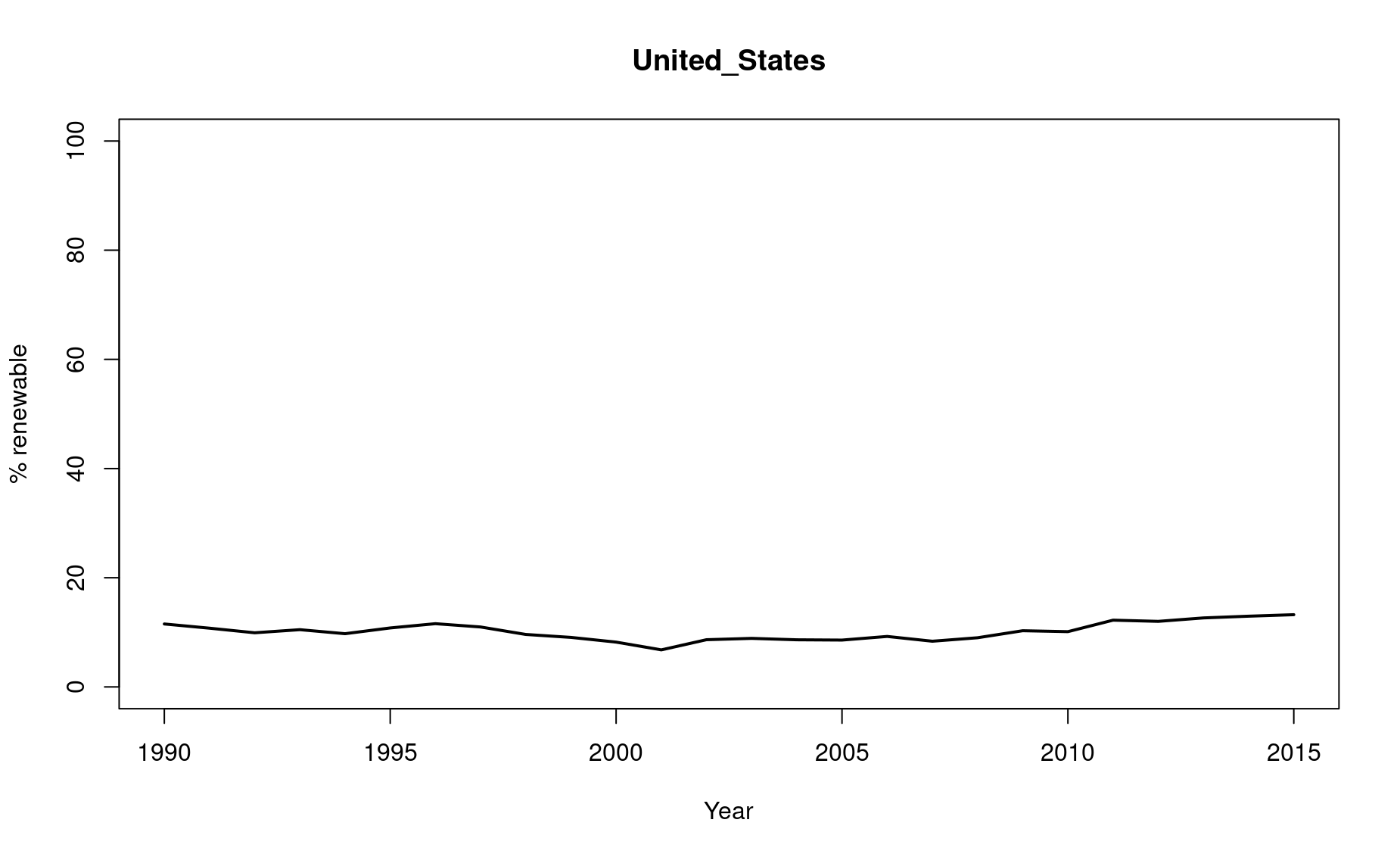
Now loop it!
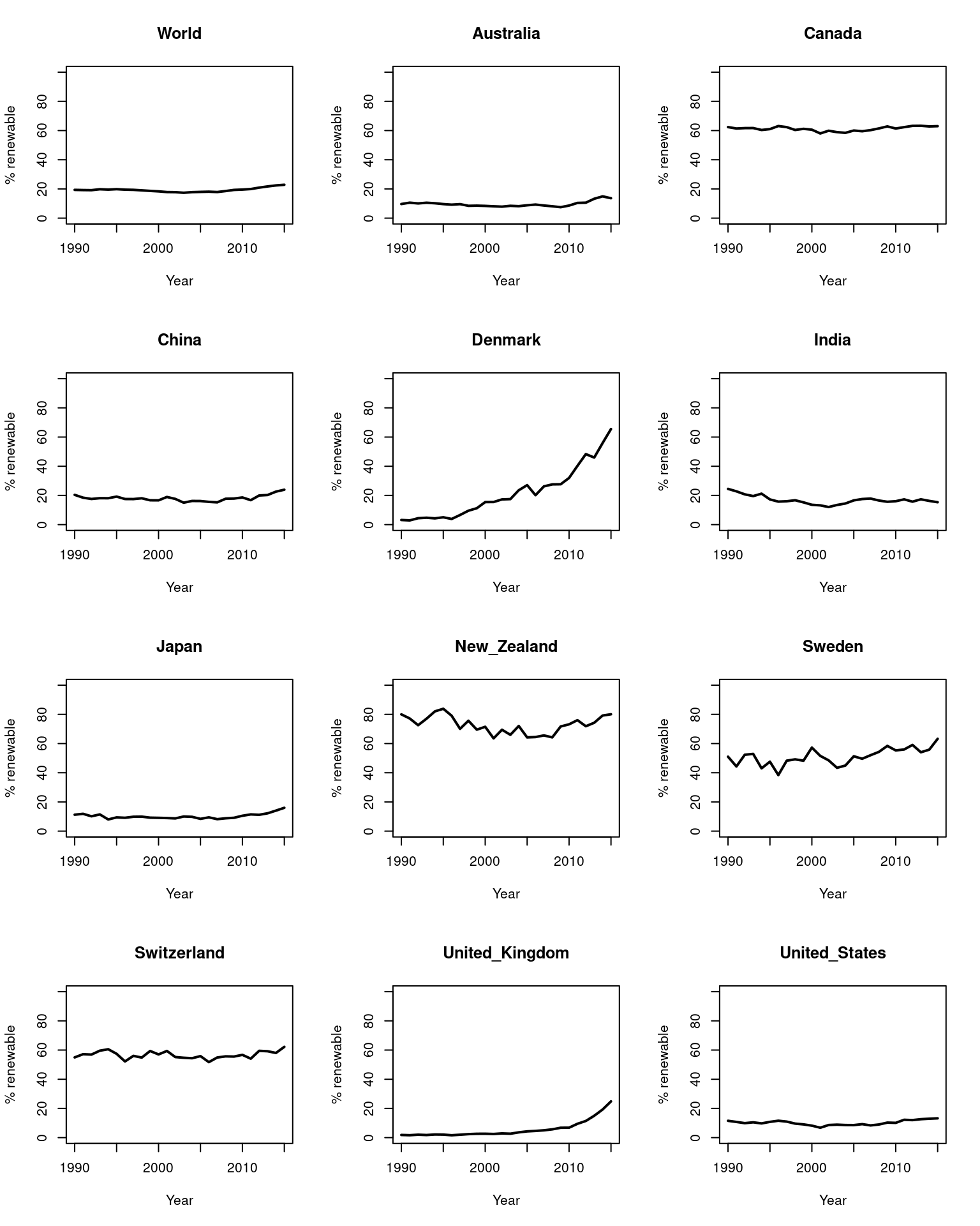
Task 3D: Use that code as the foundation for building up a for loop that displays the same time series for every country in the dataset on a multi-pane graph that with 4 rows and 3 columns.
par(mfrow=c(4,3))
i=3
for(i in 2:ncol(df)){
  dfi <- df[,c(1,i)] ; dfi
  plot(x=dfi[,1],
       y=dfi[,2],
       type="l",lwd=2,
       xlim=c(1990,2015),ylim=c(0,100),
       xlab="Year",ylab="% renewable",
       main=names(dfi)[2])
}
Now loop it in layers!
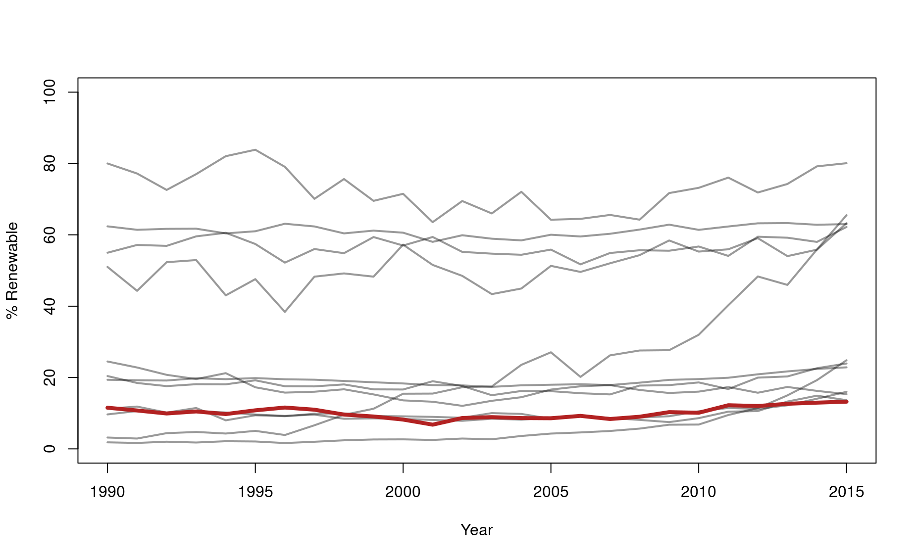
Task 3E: Now try a different presentation. Instead of producing 12 different plots, superimpose the time series for each country on the same single plot.
To add some flare, highlight the USA curve by coloring it red and making it thicker.
par(mfrow=c(1,1))
plot(1,type="n",lwd=2,
     xlim=c(1990,2015),ylim=c(0,100),
     xlab="Year",ylab="% Renewable")

for(i in 2:ncol(df)){
  dfi <- df[,c(1,i)] ; dfi
  lines(dfi[,2]~dfi[,1],lwd=2,col=adjustcolor("black",alpha.f=.4))
}

lines(df$United_States~df$year,lwd=4,col="firebrick")