Module 38 Joining datasets
Learning goals
- How to join together two related datasets efficiently in
R
It’s not unusual to have data for a project spread out across multiple datasets. The data are all related, but the fact that they are ‘packaged’ separately into different files can things difficult. To work with such relational data in R, you eventually need to merge – or join – them into a single dataframe.
For example, say you are studying the economics of professional basketball. In one dataframe, df1, you have the net worth of famous players, in millions USD…
player <- c("LeBron","Mugsy","Shaq","Jordan","Hakeem","Kobe","Stockton")
worth <- c(500, 14, 400, 1600, 200, 600,40)
df1 <- data.frame(player,worth)
df1
    player worth
1   LeBron   500
2    Mugsy    14
3     Shaq   400
4   Jordan  1600
5   Hakeem   200
6     Kobe   600
7 Stockton    40
…and in a second dataframe, df2, you have their height.
player <- c("Jordan","Shaq","Magic","Hakeem","Stockton","Mugsy","LeBron")
height <- c(78,85,81,84,73,63,81)
df2 <- data.frame(player,height)
df2
    player height
1   Jordan     78
2     Shaq     85
3    Magic     81
4   Hakeem     84
5 Stockton     73
6    Mugsy     63
7   LeBron     81
Is there a correlation between these players’ net worth and their height? To answer this question you need to join these two datasets together. But the two datasets don’t contain the exact same roster of players, and the players are not in the same order. Hmm. Is there an efficient way to join these two datasets?
Yes! Thanks to the family of join() functions from the package dplyr.
Joining with dplyr
These join() functions relate two dataframes together according to a common column name. In order for these functions to work, each dataframe has to have a column of the same name. In the case of df1 and df2, that shared column is player.
There are four join() functions you should know how to use:
left_join() joins the two datasets together, keeping all rows in the first dataframe you feed it.
left_join(df1,df2,by="player")
    player worth height
1   LeBron   500     81
2    Mugsy    14     63
3     Shaq   400     85
4   Jordan  1600     78
5   Hakeem   200     84
6     Kobe   600     NA
7 Stockton    40     73
Notice that none of the players unique to df2 made it into this output; only players in df1 (i.e., the left of the two dataframes listed) remain. Also notice that any player from df1 who was not in df2 has an NA under the column worth. That is how these join() functions work: it fills in the data where it can, and leaves NAs where it can’t.
right_join() keeps all rows in the second dataframe you feed it:
right_join(df1,df2,by="player")
    player worth height
1   LeBron   500     81
2    Mugsy    14     63
3     Shaq   400     85
4   Jordan  1600     78
5   Hakeem   200     84
6 Stockton    40     73
7    Magic    NA     81
full_join() keeping all rows in both dataframes:
full_join(df1,df2,by="player")
    player worth height
1   LeBron   500     81
2    Mugsy    14     63
3     Shaq   400     85
4   Jordan  1600     78
5   Hakeem   200     84
6     Kobe   600     NA
7 Stockton    40     73
8    Magic    NA     81
Finally, inner_join() keeps only the rows that are common to both dataframes:
inner_join(df1,df2,by="player")
    player worth height
1   LeBron   500     81
2    Mugsy    14     63
3     Shaq   400     85
4   Jordan  1600     78
5   Hakeem   200     84
6 Stockton    40     73
So, to answer our research question about the relationship between player height and net worth, we can now join these data sets and make a nice plot:
df3 <- full_join(df1,df2,by="player")
plot(df3$worth ~ df3$height,
     ylim=c(0,1700),xlim=c(60,90),
     pch=16,col="dark orange",
     xlab="Height (inches)",
     ylab="Net worth (millions USD)")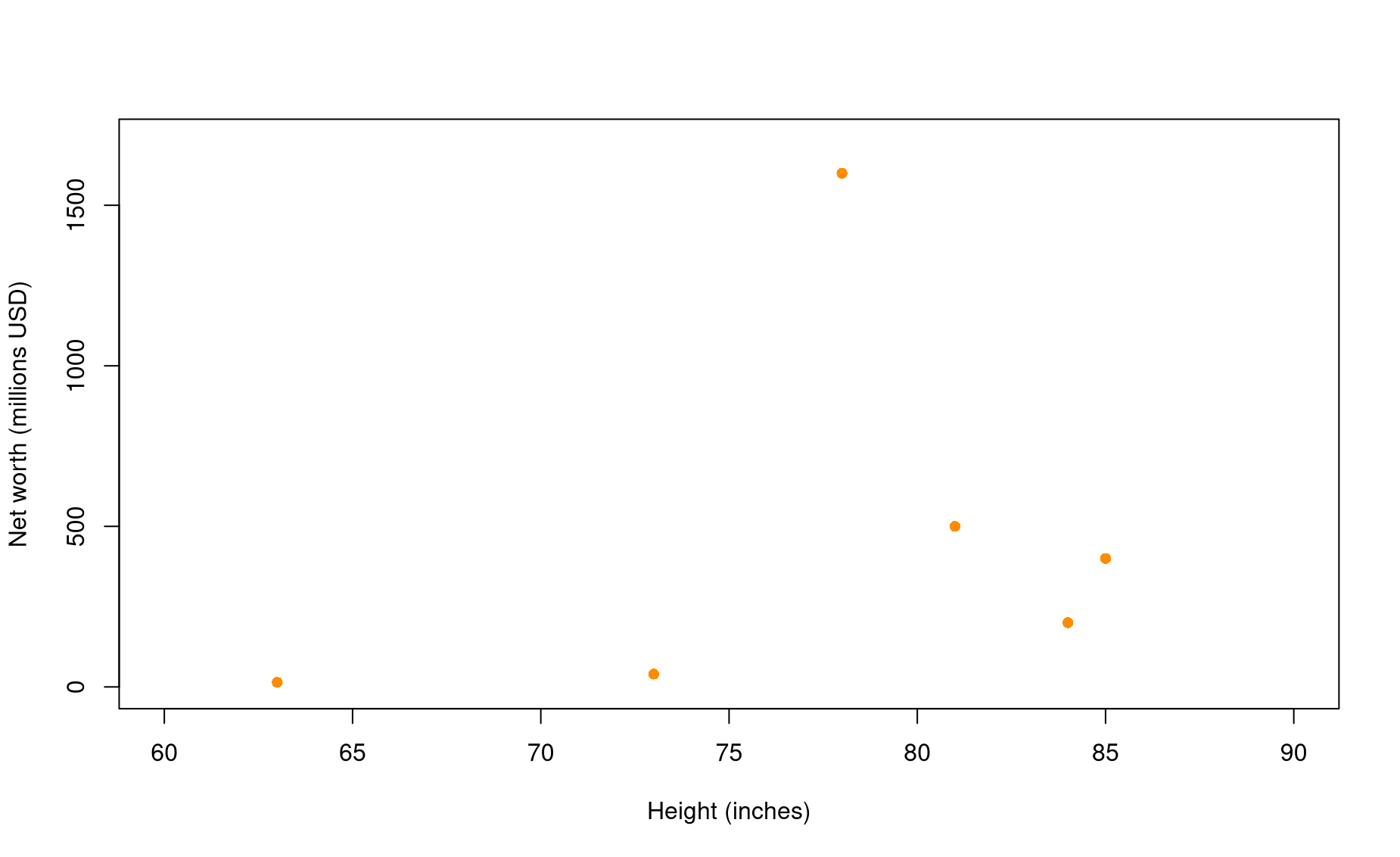
Hmm. Looks like we have an outlier!
Review exercise
This review exercise will involve both the joining skills you learned above as well as many of the skills learned in prior modules. But don’t worry: as with every exercise in this book, every puzzle here can be solved using the skills you have learned in prior modules.
Scenario: A sailing expedition conducted a survey of the whales in the fjords of British Columbia, Canada. That research produced two datasets:
env <- read.csv("./data/whales-environment.csv") ; head(env)
           id species year distance seafloor temperature salinity thermocline
1 20140811103      HW 2014  44.1021  352.881    13.49104 25.75687      9.6325
2 20140811104      HW 2014  44.2729  363.563    13.49104 25.75687      9.6325
3 20140811106      HW 2014  46.7883  361.660    13.97642 25.14305      9.7859
4 20140812102      HW 2014  44.9049  317.864    14.11392 22.26935      9.7689
5 20140812104      HW 2014  44.8370  327.717    14.12843 22.21240      9.7689
6 20140812103      HW 2014  44.6589  353.749    14.17754 22.08326      9.7426
  stratification euphotic.depth chlorophyll
1         5.0603        18.2951     81.8442
2         5.0603        18.2951     81.8442
3         5.5067        17.2179     66.1236
4         5.2032        18.0307     76.0000
5         5.2032        18.0307     76.0000
6         5.2039        18.0093     75.9543

dive <-read.csv("./data/whales-dives.csv") ; head(dive)
           id species behavior prey.volume prey.depth dive.time surface.time
1 20140811106      HW     FEED    6.914610     120.76    351.00          237
2 20140812104      HW     FEED    7.854762      79.02    281.00           87
3 20140812107      HW     FEED    7.385667      96.92    300.25           80
4 20140812109      FW     FEED    6.626298     105.87    366.00          189
5 20140812131      HW    OTHER    6.356474     123.95    357.00          112
6 20140812140      FW     FEED    3.820782     125.51    408.00          182
  blow.interval blow.number
1        26.833      10.000
2        14.412       6.667
3        16.000       6.000
4        16.273      12.000
5        25.250       6.000
6        18.789      11.000
Each row in these dataframes represent a close encounter with a whale (either a humpback whale, HW, or a fin whale, FW).
The env dataset provides details about the habitat in which the whale was found, such as seafloor depth and the amount of chlorophyll in the water (a proxy for productivity).
The dive dataset provides measurements of whale foraging behaviors, such as dive.time and the number of breaths at the surface (blow.number), as well as the quality of prey in the area (prey.volume and prey.depth).
Note that these two dataframes are linked by the id column, which is a unique code for each whale encounter.
Also note that some ids can be found in both dataframes. These are the encounters for which we have both foraging behavior data as well as environmental data.
Task 1. Summarize your dataset.
Write the necessary code and fill in the
A total of BLANK whale encounters were recorded on BLANK separate days in the years BLANK - BLANK. BLANK encounters were with humpback whales (BLANK % of all encounters), and BLANK were with fin whales (BLANK %). Foraging behavior was recorded in BLANK % of encounters (BLANK % of humpback whale encounters, and BLANK % of fin whale encounters).
Task 2. Research question: Do these two species prefer different seafloor depths?
First, create a nicely formatted histogram that portrays the data relevant to this question.
par(mar=c(4.5,4.5,3,1))
hist(env$seafloor[env$species=="FW"],
     xlab="Seafloor depth",
     main=NULL,
     prob=TRUE,
     xlim=c(0,800),
     breaks=seq(0,800,length=30),
     border=NA,
     col=adjustcolor("firebrick",alpha.f=.4))
hist(env$seafloor[env$species=="HW"],
     xlim=c(0,800),
     breaks=seq(0,800,length=30),
     border=NA,
     col=adjustcolor("darkblue",alpha.f=.4),
     prob=TRUE,
     add=TRUE)
Provide the code to test this research question statistically, then write a results statement below.
t.test(x=env$seafloor[env$species=="FW"],
       y=env$seafloor[env$species=="HW"])

    Welch Two Sample t-test

data:  env$seafloor[env$species == "FW"] and env$seafloor[env$species == "HW"]
t = 4.7677, df = 78.011, p-value = 0.000008493
alternative hypothesis: true difference in means is not equal to 0
95 percent confidence interval:
  52.84081 128.60877
sample estimates:
mean of x mean of y
 445.7157  354.9909
Task 3. Another research question: Is prey volume correlated to chlorophyll concentration?
Whales eat tiny shrimp-like critters named krill, and krill eat tiny organisms called phytoplankton. Chlorophyll is a proxy measurement for the amount of phytoplankton in the area. Based on these datasets, how good are krill at congregating in areas of high chlorophyll concentration?
First, prepare a plot to visualize what you will be comparing:
hwe <- env[env$species=="HW",] ; head(hwe)
           id species year distance seafloor temperature salinity thermocline
1 20140811103      HW 2014  44.1021  352.881    13.49104 25.75687      9.6325
2 20140811104      HW 2014  44.2729  363.563    13.49104 25.75687      9.6325
3 20140811106      HW 2014  46.7883  361.660    13.97642 25.14305      9.7859
4 20140812102      HW 2014  44.9049  317.864    14.11392 22.26935      9.7689
5 20140812104      HW 2014  44.8370  327.717    14.12843 22.21240      9.7689
6 20140812103      HW 2014  44.6589  353.749    14.17754 22.08326      9.7426
  stratification euphotic.depth chlorophyll
1         5.0603        18.2951     81.8442
2         5.0603        18.2951     81.8442
3         5.5067        17.2179     66.1236
4         5.2032        18.0307     76.0000
5         5.2032        18.0307     76.0000
6         5.2039        18.0093     75.9543
hwd <- dive[dive$species=="HW",] ; head(hwd)
           id species behavior prey.volume prey.depth dive.time surface.time
1 20140811106      HW     FEED    6.914610     120.76    351.00          237
2 20140812104      HW     FEED    7.854762      79.02    281.00           87
3 20140812107      HW     FEED    7.385667      96.92    300.25           80
5 20140812131      HW    OTHER    6.356474     123.95    357.00          112
7 20140813105      HW     FEED    7.472343     104.13    365.00           52
8 20140813107      HW     FEED    3.261088     100.19    338.00           20
  blow.interval blow.number
1        26.833      10.000
2        14.412       6.667
3        16.000       6.000
5        25.250       6.000
7        18.610       4.500
8        33.322       1.000

nrow(hwe)
[1] 446
hwe <- hwe[hwe$id %in% hwd$id,]
nrow(hwe) ; nrow(hwd)
[1] 89
[1] 89

hwe <- hwe[order(hwe$id),]
hwd <- hwd[order(hwd$id),]
hwd$chl <- hwe$chlorophyll

par(mar=c(4.5,4.5,3,1))
plot(hwd$prey.volume ~ hwd$chl,
     xlab="Chlorophyll concentration",
     ylab="Prey volume",
     pch=16,
     cex=.8)
hwlm <- lm(hwd$prey.volume ~ hwd$chl)
abline(hwlm,col="firebrick",lwd=2)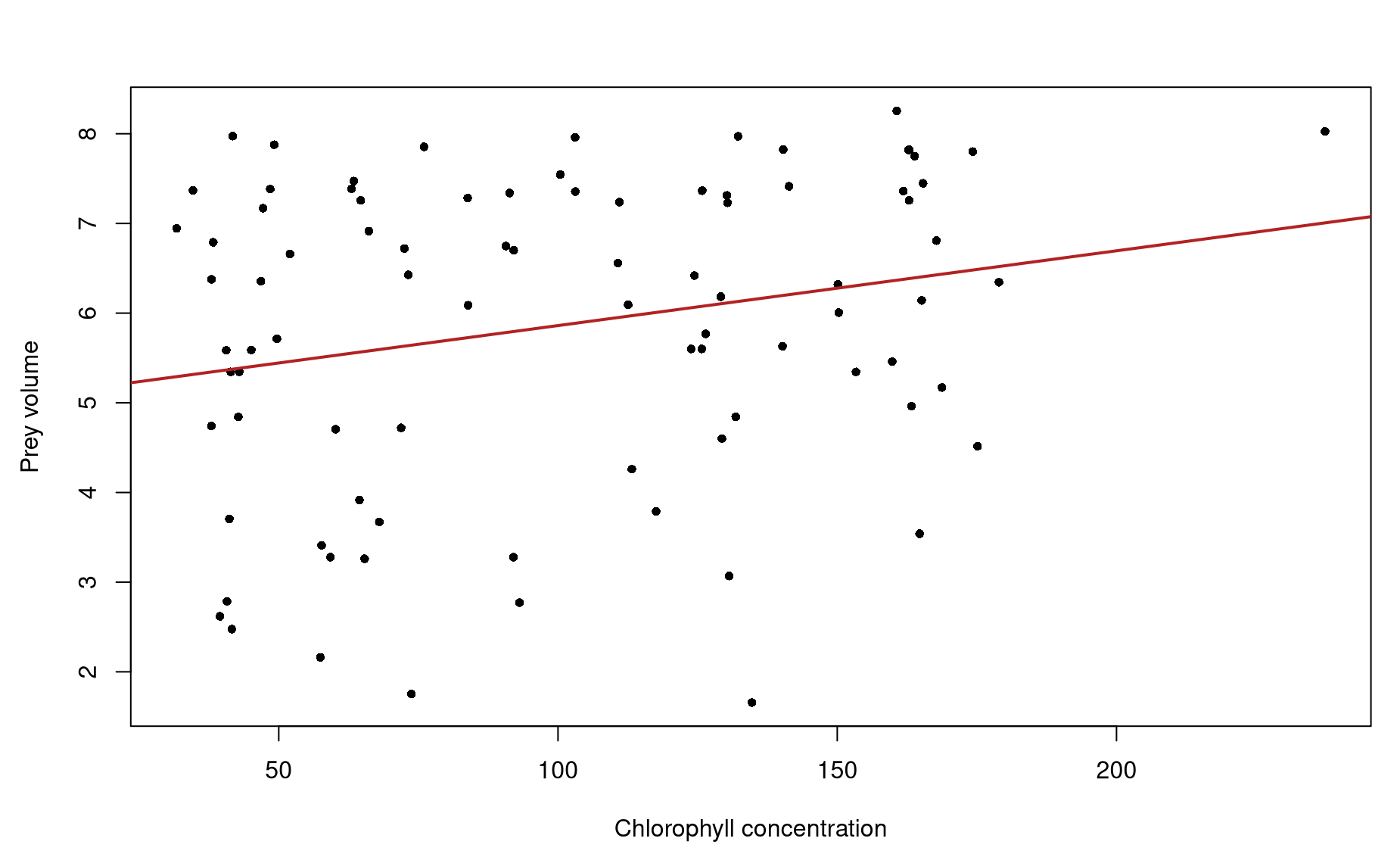
Now carry out your statistical test.
summary(hwlm)

Call:
lm(formula = hwd$prey.volume ~ hwd$chl)

Residuals:
    Min      1Q  Median      3Q     Max
-4.4931 -1.2639  0.3534  1.3358  2.5978

Coefficients:
            Estimate Std. Error t value            Pr(>|t|)
(Intercept) 5.027405   0.415675   12.10 <0.0000000000000002 ***
hwd$chl     0.008340   0.003723    2.24              0.0276 *
---
Signif. codes:  0 '***' 0.001 '**' 0.01 '*' 0.05 '.' 0.1 ' ' 1

Residual standard error: 1.682 on 87 degrees of freedom
Multiple R-squared:  0.05453,   Adjusted R-squared:  0.04366
F-statistic: 5.018 on 1 and 87 DF,  p-value: 0.02763