Module 47 Writing functions
Learning goals
- Be able to write your own functions
- Be able to use functions to make your work more efficient, effective, and organized
First steps
You’ve already used dozens of functions during your learning in R so far. As you start applying R to your own projects, you will inevitably encounter a puzzle that could be solved by a custom function you write yourself. This module shows you how.
As explained in the Calling Functions module, most functions have three key components:
- one or more inputs,
- a process that is applied to those inputs, and
- an output of the result.
When you define your own custom function, these are the three pieces you must be sure to include.
Here is a basic example:
Now use your function:
Let’s break this down.
my_functionis the name you are giving your function. It is the command you will use to call your function.- The
function()command is what you use to define a function. xis the variable you are using to represent your input.y <- 1.3x + 10is the process that you are applying to your input.return(y)is the command you use to define what the function’s output will be.
Note that you are not required to write out x=2 in full when you are calling your function. Just providing 2 can also work:
Next steps
Multiple inputs
You can define a function with multiple inputs. Just separate each input with a comma.
To demonstrate this, let’s modify the function above to allow you to define any linear regression you wish:
Now call your function:
Note that you do not need to write out the name of each input, as long as you provide inputs in the correct order.
But note that it is usually best practice to name each input in your function call, to prevent the possibility of any confusion or mistakes. Also, when you name each input you can provide inputs in whatever order you wish:
Providing defaults for inputs
Just as R’s base functions include default values for some inputs (think na.rm=FALSE for mean() and sd()), you can define defaults in your own functions.
This version of my_function includes default values for inputs a and b.
When you provide default values, you no longer need to specify those inputs in your function call:
Adding plots
Plots can be included in the function commands just as in any other context:
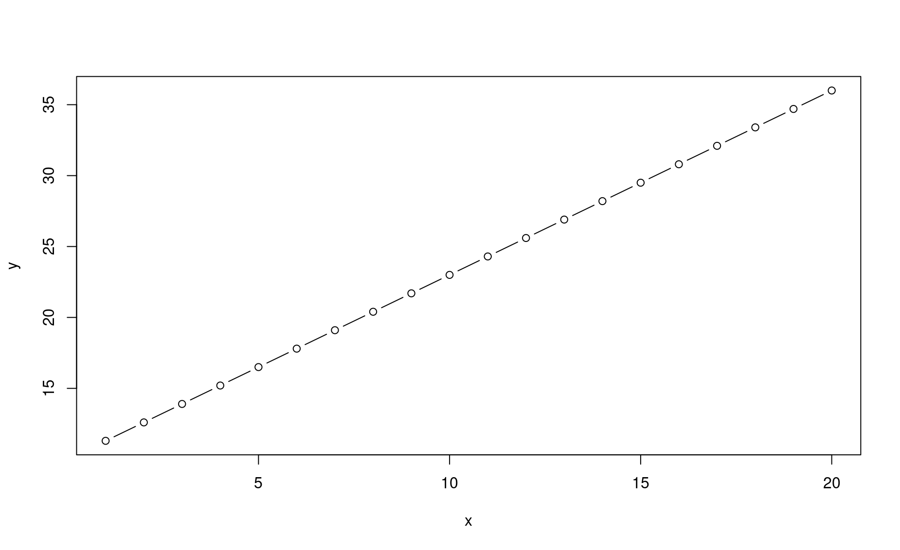
 [1] 11.3 12.6 13.9 15.2 16.5 17.8 19.1 20.4 21.7 23.0 24.3 25.6 26.9 28.2 29.5
[16] 30.8 32.1 33.4 34.7 36.0
Adding plots to functions can be super useful if you want to make multiple plots with the same formatting specifications. Rather than retyping the same long plot commands multiple times, just write a single function and call the function as many times as you wish.
Let’s add some fancy formatting to our plot. Note that we will modify the name of the function to make it more descriptive and helpful. The lm in plot_my_lm stands for linear model, which is what is being defined with the y=ax+b equation.
plot_my_lm <- function(x,a=1.3,b=10,plot_only=TRUE){

  # Process
  y <- a*x + b

  # Plot
  par(mar=c(4.2,4.2,3,.5)) # set plot margins
  plot(y ~ x, type="o",axes=FALSE,ann=FALSE,pch=16,col="firebrick",xlim=c(-20,20),ylim=c(-20,20)) # define basic plot
  title(main=paste("y =",a,"x +",b)) # print a dynamic main title
  title(xlab="x",ylab="y")  # print axis labels
  axis(1) # print the X axis
  axis(2,las=2) # print the Y axis and turn its labels right-side-up
  abline(h=0,v=0,col="grey70") # add grey lines indicating x=0 and y=0

  # Return
  if(plot_only==FALSE){
    return(y)
  }
}
Note that we added a parameter, plot_only. When it is set to TRUE, the function will not return any numbers.
Now let’s call this fancy function a bunch of times:
my_input <- -20:20 # define a common x input value

par(mfrow=c(3,2)) # stage a multi-paned plot
plot_my_lm(x=my_input,a=2,b=15)
plot_my_lm(x=my_input,a=1,b=10)
plot_my_lm(x=my_input,a=.5,b=5)
plot_my_lm(x=my_input,a=0,b=0)
plot_my_lm(x=my_input,a=-1,b=-5)
plot_my_lm(x=my_input,a=-2,b=15)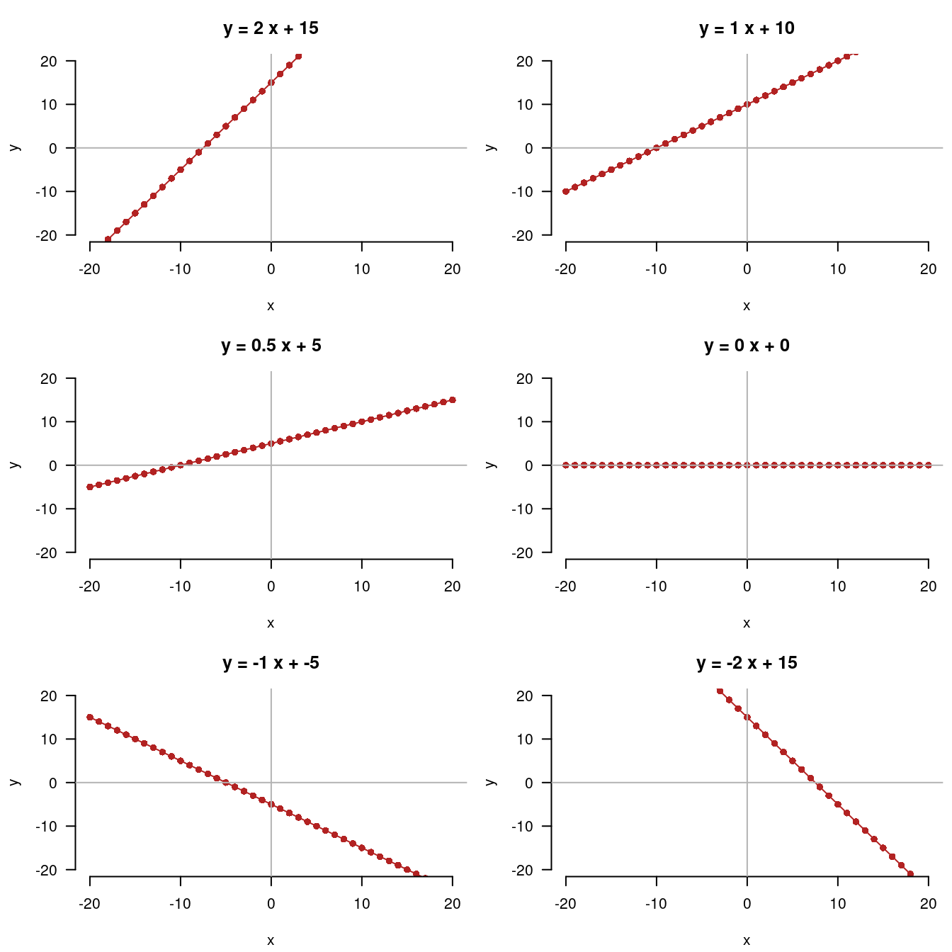
Think about how many lines of code would have been needed to write out all of these fancy plots if you did not use a custom function! Think about how cluttered and dizzying your code would look! And think about how many opportunities for errors and inconsistencies there would have been! That is the advantage of writing your own functions: it makes your work more efficient, more organized, and less prone to errors.
Another major advantage of this approach comes into play when you decide you want to tweak the formatting of your plot. Rather than going through each plot(...) command and modifying the inputs in each one, when you write a custom plotting function you just have to make those changes once. Again, using a custom function saves you time and removes the possibility of inconsistencies or mistakes in the plots you are creating.
Exercises
Modify the most recent version of plot_my_lm above such that you can specify the color for the plotted line as an input in the function. Then reproduce the multi-paned plot using a different color in each plot. (Here is a good reference for color options in R).
Sourcing functions
As you advance in your coding, you will likely be writing multiple custom functions within a single R script. It is usually useful to group these functions into the same section of code near the top of your script.
But for even better script organization and simplification, you should source your functions from a separate R script. This means placing your function code in a separate R script and calling that file from the script in which you are carrying out your analyses. In addition to simplifying your analysis script, keeping your functions in a separate file allows them to be shared or sourced from any number of other scripts, which further organizes and simplifies your project’s code and increases the reproducibility of your work.
Here is how sourcing functions can work:
Open a new
Rscript. Save it asfunctions.Rand save it in the same working directory as the script you are using to work through this module.Copy and paste the
plot_my_lm()function into yourfunctions.Rscript. Save that script to ensure your code is safe.Now remove the code defining
plot_my_lm()from your moduleRscript.In its place, type this command:
This command tells R to run the code in functions.R and store the objects and outputs from it in its active memory. You can now call plot_my_lm() from your module script.
Review exercises
Carry out the above instructions to ensure that you know how to source a function from a separate R script.
Exercises with baby names
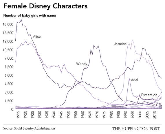
In this exercise, you will investigate annual trends in the prevalence of six names for babies born in the United States.
1. Decide upon five names of interest to you, in addition to your own. Create a vector of these six names.
2. Install and load the package babynames, which includes the names of each child born in the United States from 1880 to 2017, according to the Social Security Administration.
3. Make an object named bn like this: bn <- babynames::babynames.
4. Write a function that takes any name and plots its proportional prevalence from 1880 to 2017. Format the plot beautifully. Provide the name as the title of the plot.
5. Modify your function so that it takes multiple names (instead of just one) and generates a multi-pane plot, one for each of the names passed to the function. Then, test that function on the object you created in number one.
6. Create a function called first_letter. This should take any vector as an argument and return the first letter only. You will need to use the substr function.
7. Use your first_letter function to make a new variable in the babynames dataset called fl. This should be the first letter of all names.
8. What was the most popular first letter of boys names in 1900?
9. What was the least popular first letter of girls names in 2017?
10. Make a function called letter_plot. This should take two arguments, letter and m_or_f, and then create a plot showing the popularity of that letter for the letter/sex combination inputted over time.
11. Make a function called letter_compare. This should take two arguments: y (the year) and gender (sex). This should make a plot of the popularity of each letter being used as the first letter for a name, for the sex in question, for the year provided.
Exercises with trees data
12. Define an object named trees using the built-in trees dataset: trees <- trees (weird, right?)
13. How many rows are there?
14. How many columns are there?
15. “Girth” is the same thing as “circumference”. Make a function named girth_to_diameter. It should do exactly what it says.
16. Create a new variable called diameter. Use your new function to populate it.
17. Create a scatterplot showing the association between diameter and Volume.
18. Create a histogram of Height.
19. Create a function named diameter_to_area. It should do what it says it does. Create a new variable named area using this function. This should be the area of a cross-sectional cut of the tree.
20. Create a dataset named oranges by reading in the built-in Orange dataset like this: oranges <- Orange.
21. Create a plot showing circumference as a function of age, faceted by tree number.
22. Create a function called plot_tree. This should take only one argument, tree_number, and generate a plot of that tree’s growth over time.
23. Create a function called circumference_to_radius. It should do what it says. Use it to create a new variable in the oranges data named radius.
24. Create a function called double_it. It should double it. Use it to create a variable named diameter.
25. Assume that the measurements of the trees are in inches, and that the age of the trees is in days. Create (a) a function for converting inches to centimeters and (b) a function for converting days to weeks. Create new variables in the data, using these functions, named circumference_cm and age_weeks.
26. Plot the association between age in weeks and circumference in centimeters. Facet by tree number.
27. Do trees get bigger as they get older?
Exercises with dplyr and ggplot
Previously we analyzed and explored the dataset by using dplyr and ggplot. A lot of our analysis used the same code, just applied to different variables and aspects of the data.
# plot the gdp per capita for china over time
china_gdp <- gm %>% filter(country == 'China')
ggplot(china_gdp, aes(year, gdpPercap)) +
  geom_line() +
  labs(x = 'Year', y = 'GDP per capita', title = "China GDP per capita over time")

# now india
india_gdp <- gm %>% filter(country == 'India')
ggplot(india_gdp, aes(year, gdpPercap)) +
  geom_line() +
  labs(x = 'Year', y = 'GDP per capita', title = "India GDP per capita over time")
If we want to do this for every country we will be reusing the same code over and over again. Lets write a function
plot_gdp <- function(country_name){
  plot_data <- gm %>% filter(country == country_name)
  ggplot(plot_data, aes(year, gdpPercap)) +
    geom_line() +
    labs(x = 'Year', y = 'GDP per capita', title = paste0(country_name, ' GDP per capita over time'))
}
plot_gdp(country_name = 'China')
plot_gdp(country_name = 'India')
plot_gdp(country_name = 'Angola')
Lets take it a step further and add a plotting variable
plot_gdp <- function(country_name, plot_var){
  plot_data <- gm %>% filter(country == country_name)
  ggplot(plot_data, aes_string('year', plot_var)) +
    geom_line() +
    labs(x = 'Year', y = plot_var, title = paste0(country_name,' ', plot_var ,' over time'))
}
plot_gdp(country_name = 'China', plot_var = 'pop')
plot_gdp(country_name = 'India', plot_var = 'lifeExp')
plot_gdp(country_name = 'Angola',plot_var = 'gdpPercap')
Now keep going:
28. Create a function that filters by a continent and year and creates a barplot of the population for all the countries in that continent
29. Add a color argument to the function called color_bars that fills the bar chart with that color
30. Add a title argument to the function that’s called plot_title that combines the name and year into the title of the plot
31. Add another argument that specifies the numerical variable you are plotting on the y axis (up until now it was just population. hint(aes_string))
32. Add another argument called plot_type that has a default value “bar”. Use conditionality (if and else statements) to create a bar chart if plot_type=“bar”, a point plot otherwise.
33. Create your own function that filters the data in some way and makes a plot. The function should have at least 5 arguments.